25 min read

This article contains details on sim2real in robotic manipulation for following tasks:

Perception for manipulation (DOPE / SD-MaskRCNN).
Grasping (Dex-Net 3.0 / 6DOF GraspNet).
End-to-end policies. (Contact rich manipulation tasks & In hand manipulation of rubik’s cube)
Guided domain randomization techniques (ADR / Sim-Opt).

The reality gap:

An increasingly impressive skills have been mastered by DeepRL algorithms over the years in simulation (DQN / AlphaGo / OpenAI Five). Both Deep learning and RL algorithms require super huge amounts of data. Moreover, RL algorithms there is risk to the environment or to the robot during the exploration phase. Simulation offers the promise of huge amounts of data (can be run in parallel and much faster than real time with minimal cost) and doesn’t break your robot during exploration. But these policies trained entirely in simulation fails to generalize on real robot. This gap between impressive performance in simulation and poor performance is known as the reality gap.

Some of the ways to bridge the reality gap are:

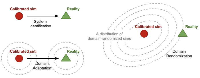
Illustration of Sim2Real Approaches. PC: Lil’Log [1]

System Identification: Identify exact physical / geometrical / visual parameters of environment relevant to task and model it in simulation.
Domain Adaptation: Transfer learning techniques for transferring / fine-tuning the policies trained in simulation in reality.
Domain Randomization: Randomize the simulations to cover reality as one of the variations.

We’ll mainly be focussing on domain randomization techniques and their extension used in some of the recent and successful sim2real transfers in robotic manipulation.

Domain Randomization

Formally domain randomization is defined as:

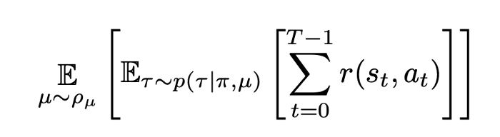
P_{mu} is the randomized transition distribution. τ is the trajectory of samples as per policy π in the environment P_{mu}.

So effectively, domain randomization is trying to find a common policy π parameters that work across a wide range of randomized simulations P_{mu}. So the hope is that the policy that works across wide range of randomizations also works in the real world, assuming that the real world is just another randomization covered by randomization.

Based on how these simulation randomization are chosen we have 2 types:

Domain randomization: Fixed randomization distributions over a range often chosen by hand. We will see how this has been used in perception & grasping tasks for data efficiency.
Guided domain randomization: Either simulation or real world experiments can be used to change the randomization distribution. We will see how this has been used in training end2end policies for contact rich and dexterous tasks. Some of the guided domain randomizations do appear like domain adaptation.

Domain randomization:

Some of the early examples of using domain randomizations was used for object localization on primitive shapes[2] and table top pushing[3]. We will look at examples of more advanced tasks such as segmentation and pose estimation with emphasis on what randomizations were chosen and how good are the transfer performance.

Domain Randomization in Perception:

SD Mask R-CNN: SD (Synthetic Data) Mask R-CNN trains category agnostic instance segmentation entirely based on synthetic dataset with performance superior to that fine-tuned from COCO-dataset.

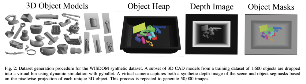
Data Generation Procedure for SD-Mask-RCNN. WISDOM (Wear House Instance Segmentation Dataset for Object Manipulation).

Simulator: pybullet

Randomizations: Since this network uses depth images as inputs, the randomizations needed are quite minimal ( depth realistic images are easy to generate compared to photo realistic).

Sample a number n ∈ p(λ = 5) of objects and drop it in the bin using dynamic simulation. This will sample different objects and different object poses.
Sample camera intrinsics K and camera extrinsic (R, t) ∈ SE(3) within a neighborhood of real camera intrinsics and extrinsic setup.
Render both the depth image D and foreground object masks M.

The Mask-RCNN trained on instance segmentation entirely on synthetic data (SD-Mask R-CNN) is compared against a couple of baseline segmentation methods and Mask R-CNN trained on COCO dataset & fine-tined (FT Mask R-CNN) on WISDOM-real-train. The test set WISDOM-real-test used here is the real world dataset collected using a high-res and low-res depth cameras and hand labelled segmentation masks.

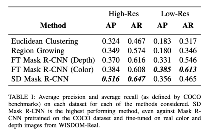
Performance of Mask R-CNN. For both AP (Average Precision) and AR (Average Recall) higher is better.

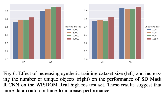
From the ablation study, both metrics go up as number of synthetic data samples are increased indicating more data could help the improve the performance. However, increasing the number of unique objects has mixed results (may be due limited number of objects in WISDOM-real-test).

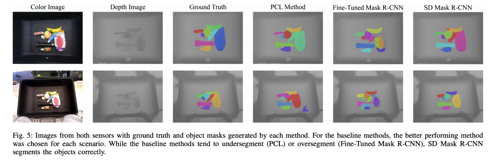
Some qualitative comparison of segmentation results from SD Mask R-CNN

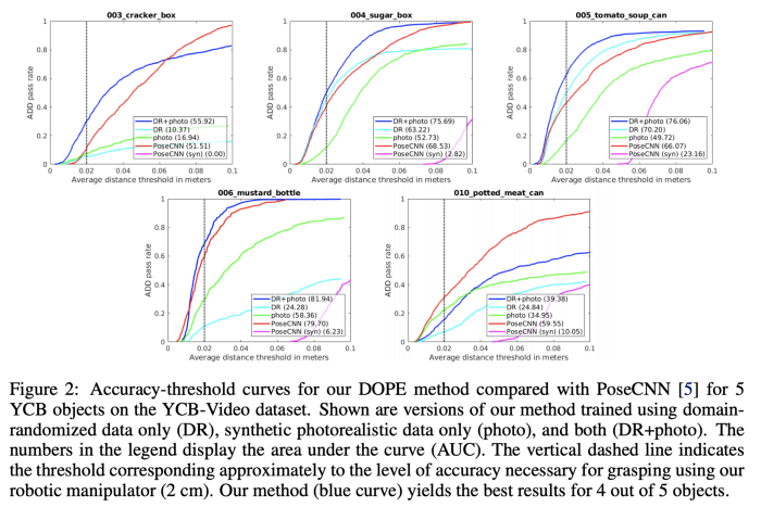
DOPE (Deep Object Pose Estimation): DOPE solves the problem of pose estimation of YCB objects entirely using synthetic dataset that contain domain randomized and photorealistic RGB images.

Simulator: UE4 with NDDS Plugin.

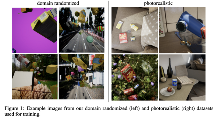
Domain Randomizations:

Number of / types / 3D poses / textures on distractor objects of primitive 3D shapes.
Numbers / textures / 3D poses of objects of interest from YCB objects set.
Uniform / textured or images from COCO as background images.
Directional lights with random orientation and intensity.

Photorealistic:

Falling YCB objects in photo realistic scenes from standard UE4 virtual environments. These scenes are captured with different camera poses.

Notice that camera intrinsics randomization wasn’t necessary here since the method regresses heat-maps of 3D box and vector fields to the centroid. It uses these predicted 2D information / camera intrinsics (explicitly) / object sizes to predict the 3D pose.

ADD (Average distance of 3D points on bounding boxes) pass rate vs distance threshold plots below measures successful pose detection within that threshold (higher is better). Notice how both DR and photorealistic images were necessary to get comparable performance to method trained on real world data (PoseCNN).

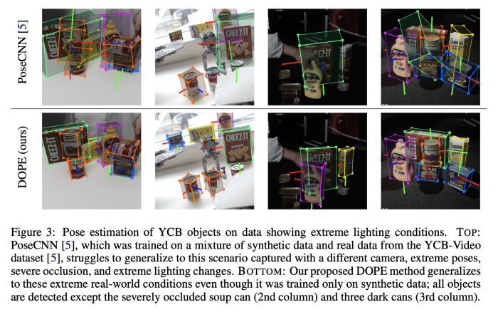
Some qualitative comparisons of DOPE with PoseCNN (real data) is shown below. Notice how DOPE produces tighter boxes and more robust to lighting conditions.

Domain Randomization in Grasping:

Let’s look at some examples of domain randomizations applied to robotic grasping (both suction based and parallel jaw grasps) with emphasis on what aspects are randomized and their transfer success to real robot grasping.

Dex-Net 3.0:

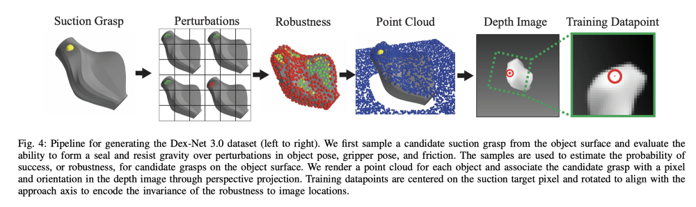
Suction GQ(Grasp Quality)-CNN takes in a depth image patch centered at suction point and outputs a quality measure. The process of generating the quality measure labels is illustrated below:

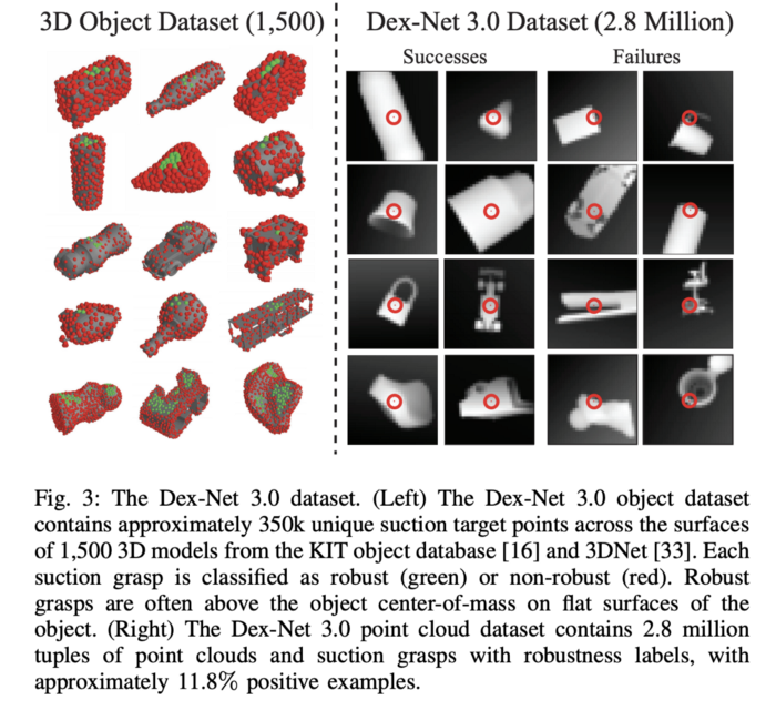
Here are examples of few more labels generated with grasp robustness annotated 3D models:

Simulator: Custom quasi-static physics model that simulates seal formation and ability to resist gravity and random external wrenches.

Randomizations: The graphical model shows the randomization parameters used in Dex-Net 3.0

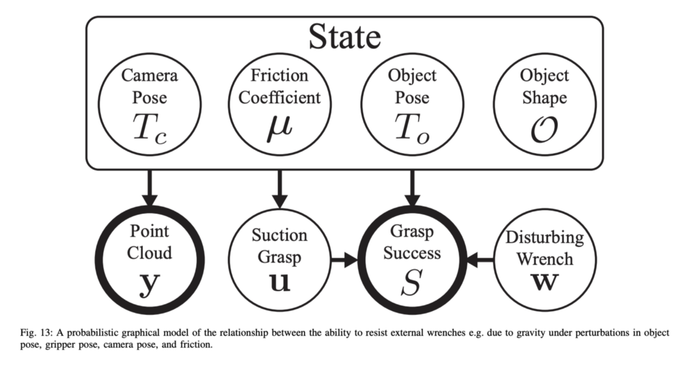
PC: Dex-Net 3.0

Here are the randomizations explicitly listed:

Sample a 3D object O uniformly from training set.
Sample a resting pose T_s and sample planar disturbance from U([-0.1, 0.1], [-1.0, 1.0], [0, 2π)) and apply the planar disturbance (x, y, θ) to T_s to obtain object pose T_o
μ coefficient of friction is sampled from N_+(0.5, 0.1)
Camera pose T_c is sampled in spherical coordinates (r, θ, ϕ) ∈ U([0.5, 0.7], (0, 2π, 0.01π, 0.1π)) where the camera optical axis intersections the table.
Suction grasps are uniformly sampled on object 3D mesh surface.

For each such sampled grasp, the wrench resistance metric is computed and the point cloud for the 3D object mesh is rendered using sampled camera pose and known camera intrinsic.

Zero shot transfer of policy (CEM) that optimizes the samples according to suction GQ-CNN is shown in video below:

6DOF GraspNet:

The GraspNet framework has 2 components both of which take the point cloud corresponding to target object:

VAE (Variational Auto-Encoder) predicts 6-DOF grasp samples that has high coverage on the target object.
Grasp evaluator that takes 6-DOF grasp sample in addition to point cloud produced quality scores. Which is later used for refining the grasp sampled via VAE.

The gradient on the grasp evaluator can be used to further refine the sampled grasps.

Training both networks require positive grasp labels, which are generated entirely in simulation.

Simulator: NVIDIA FleX simulator.

Synthetic grasp data generation:

An object is sampled from a subset of ShapeNet.
An approach based sampling scheme is used for generating grasp samples. Samples that are not in collision and non-zero object volume are selected for simulation.
Object mesh and gripper in the sampled pose are loaded in simulation. Surface friction and object density are kept constant (No randomizations ! really ?). The gripper is closed and a predefined shaking motion is executed. Grasps that keep the object between the grippers are marked as positive grasps.
Hard negative grasps are generated in neighborhood of positive grasps that are either in collision with gripper or zero object volume between grippers.

The visualization of the grasp data generation:

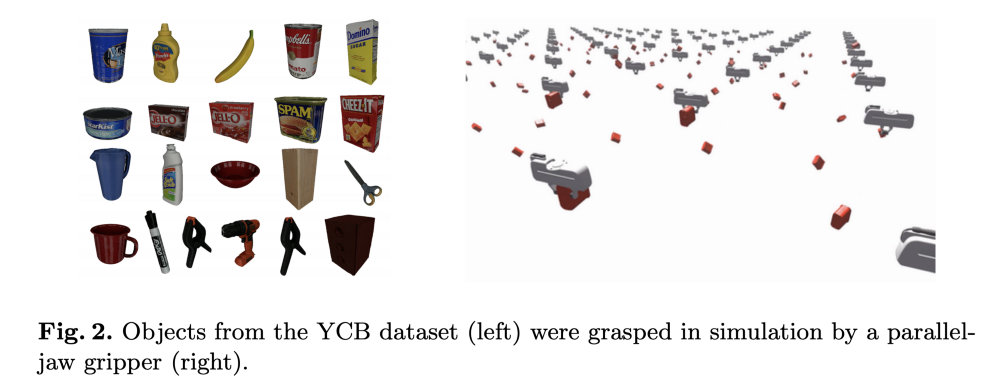
Note that 6-DOF GraspNet doesn’t actually use YCB objects for training. This is just for illustrating the data generation process. PC: Billion ways to grasp

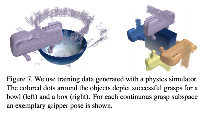
Some of the positive grasp samples on bowls and boxes are shown below:

The performance of 6-DOF GraspNet on previously unseen YCB objects:

Guided domain randomization:

Previously, we saw several examples of randomized simulations that lead to successful transfer to real robotic tasks. These randomizations were chosen carefully around the nominal real world values and often tuned for real world transfer. This either becomes tedious when there are large number of parameters to choose for and very wide randomizations often leads to infeasible / sub-optimal solutions in simulations. We will look at two strategies for automating this:

Automatic domain randomization in the context of solving Rubik’s code.
Sim-Opt in the context of contact rich manipulation tasks which uses real world rollouts of policy.

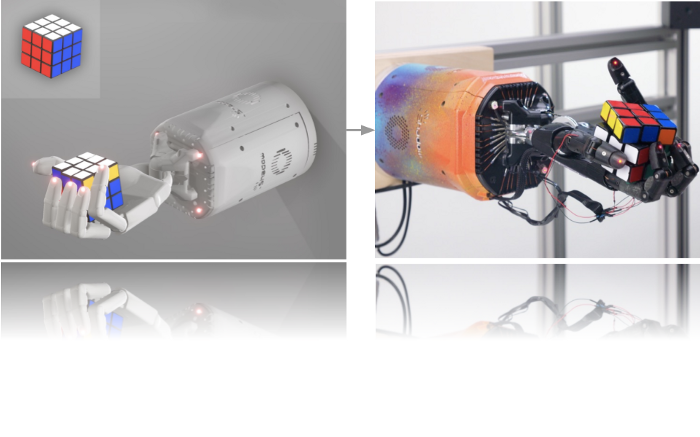
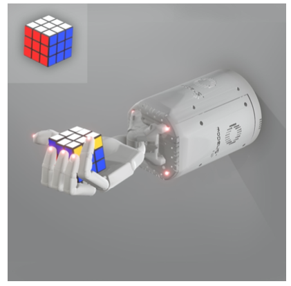
Automatic Domain Randomization (ADR):

Let’s take a brief look at the overall framework used for Rubik’s cube solving before delving into ADR algorithm. Here is a nice overview of the entire framework:

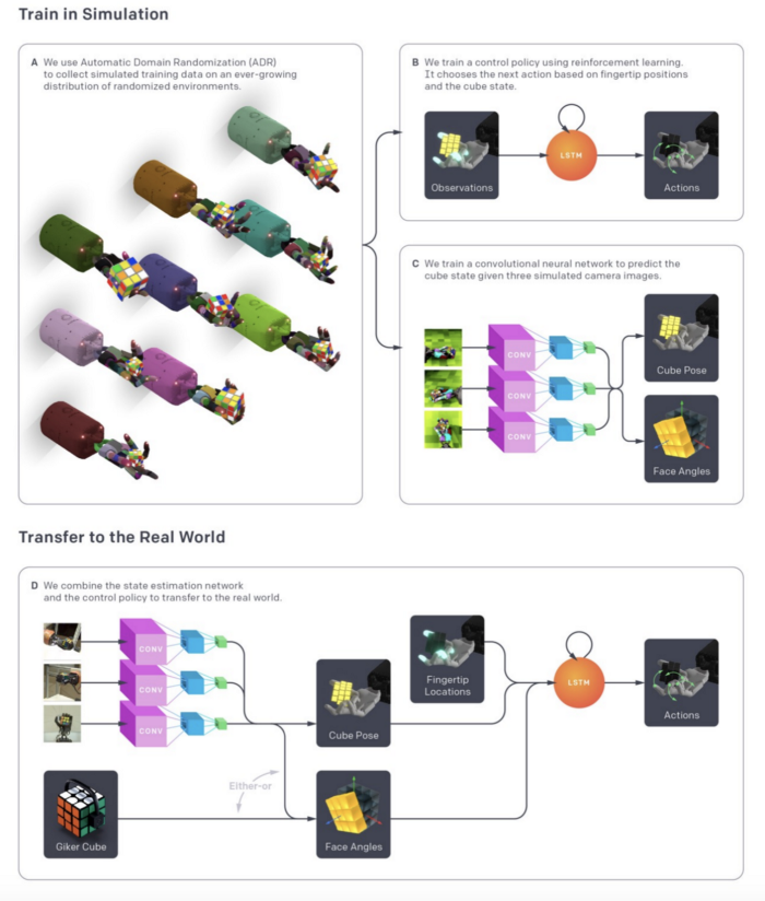
Overview of framework for solving the Rubik’s cube. Giiker is a “smart” Rubik’s cube that has sensing of face angles upto 5⁰ resolution.

Although, the vision part of network is also trained entirely in simulation with ADR , let’s focus on hard controller policy part that manipulates the Rubik’s cube. Note that optimal sequence of rotations of Rubik’s cube faces are solved by Kociemba’s algorithm

The task of solving the Rubik’s cube now reduces to the problem of successfully executing face rotations and flip actions to make sure the face to be rotated is on top.

The shadow robotic hand is used for performing the flip and rotations on the Rubik’s cube. Here are the details of inputs and outputs of the policy network and reward functions.

Inputs: Observed fingertip positions, observed cube pose, goal cube pose, noisy relative cube orientations, goal face angles, noisy relative cube face angles.

Outputs: shadow hand has 20 joints that can be actuated, and the policy outputs a discretized actions space of 11 bins per joint.

Reward function: Combination of:

Distance between present cube state to goal state.
Additional reward for achieving the goal.
Penalty for dropping the cube.

Also, episodes are terminated based on 50 consecutive successes / dropping the cube or time out while trying to achieve the goal.

Simulator: MuJoCo

Also, a lot of effort has been put into simulating the details of Rubik’s cube dynamics and Shadow robot hand.

Visualization of Rubik’s cube task in MuJoCo simulator.

ADR Algorithm:

Compared to naive domain randomization:

Curriculum learning: ADR gradually increases the task difficult leading easier policy converge.
Automatic: Removes the need for manual tuning of parameters, that could be non-intuitive for large parameter set.

Randomizations:

Simulator physics parameters such as friction between cube, robot hand, cube size, parameters of the hand model etc.
Custom physics parameters such as action latency, time step variance.
Observation noise to cube poses, finger positions at episode level as well as each step level.

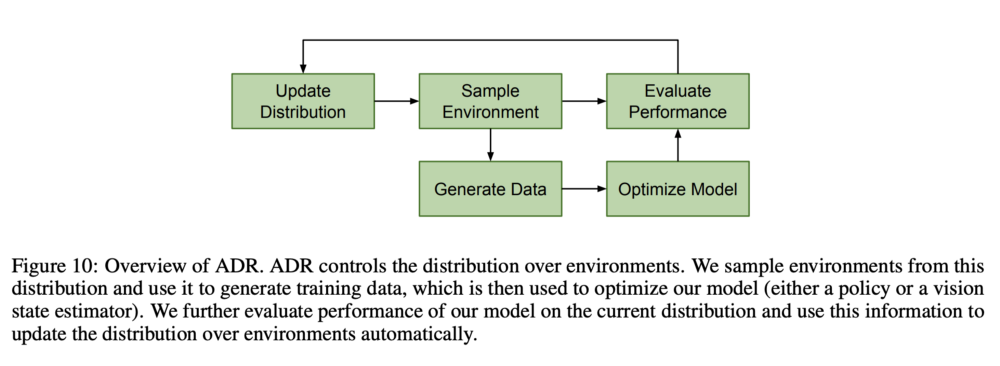
Overview of ADR

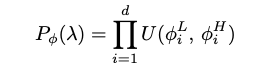
All simulation parameters are sampled from uniform distribution over a range (ϕ_L, ϕ_H). Thus is distribution of simulator parameters for d parameters is given by:

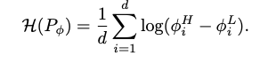
And entropy is used for measuring the complexity of training distribution, which for product of uniform distribution is:

Task performance (i.e number of success in a given episode) thresholds (t_L, t_H) is used to adjust the parameters ϕ. ADR starts with a single simulation parameter value. At each iteration, one of the boundary (ϕ_L or ϕ_H) value of one of the randomization parameter ϕ_i is chosen and the performance is evaluated and added to a buffer (D_L or D_H). After the buffer is of adequate size, depending on whether the overall performance is above t_H or below t_L, ϕ_i range is increased or ϕ_i range is decreased respectively.

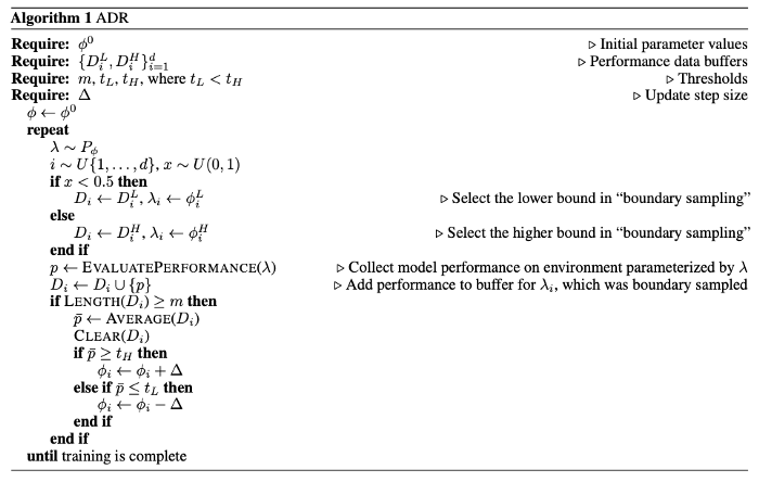
Detailed algorithm for ADR

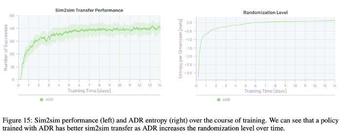
Sim2Sim: The benefit of curricular learning was studied in the context of Sim2sim transfer of bringing the cube to goal orientation. The test set is previously hand tuned domain randomization scheme which was never presented to ADR. As can be seen, as the entropy of domain randomization goes up, as does the performance on the test simulation environment.

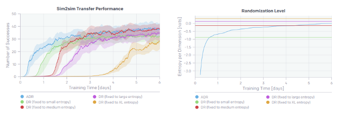
ADR is compared against several fixed randomization schemes that were reached via curriculum training, as can be seen ADR reaches higher performance quickly and asymptotically similar.

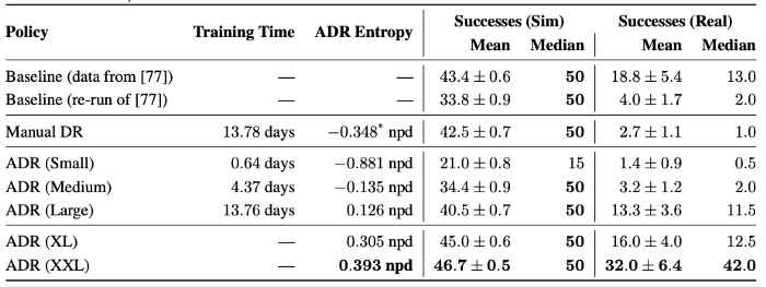
Sim2Real: The table below shows performance of ADR trained policy in Sim and in Real for different amounts of training. Notice how the entropy of P_ϕ keeps growing as the training progresses.

Here is a successful execution of solving the Rubik’s cube from a random shuffle:

Meta-learning perspective: Because the LSTM policy doesn’t have enough capacity to remember all the variations of dynamics, it learns to adapt the policy to particular instantiations of dynamics during execution (i.e online system identification).

This is studied by perturbing the memory of LSTM / changing the dynamics on the fly or restraining a random joint. As can be seen each of the perturbations, the amount of time needed to complete the sub-goal suddenly goes up as the perturbation is introduced and after several executions the policy calibrates itself to new dynamics and the performance returns to it’s corresponding baseline.

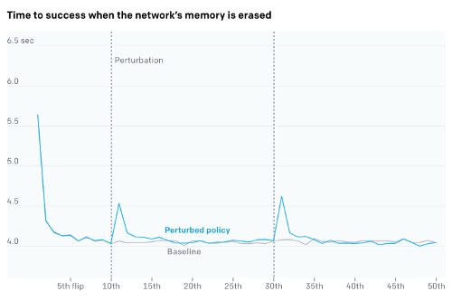
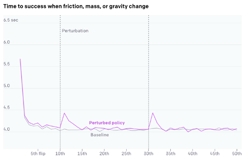
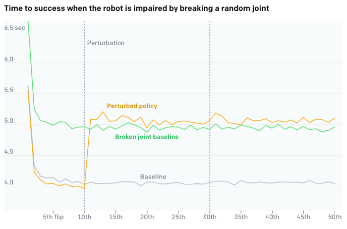
Plots showing the online system identification effects.

Sim-Opt:

Sim-opt framework is trying to find parameters of simulation distribution that makes discrepancy between observed trajectory in simulation vs in real world by executing the trained policy.

It showcases the approach with two real world robotic tasks on two separate robotic hands:

Drawer opening with Franka Emika Panda.
Swing peg in hole task with ABB YuMi.

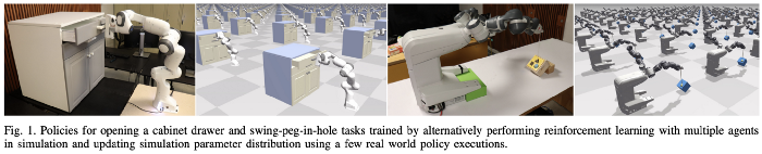
Tasks solved by Sim-Opt

Here is the overview of SimOpt framework:

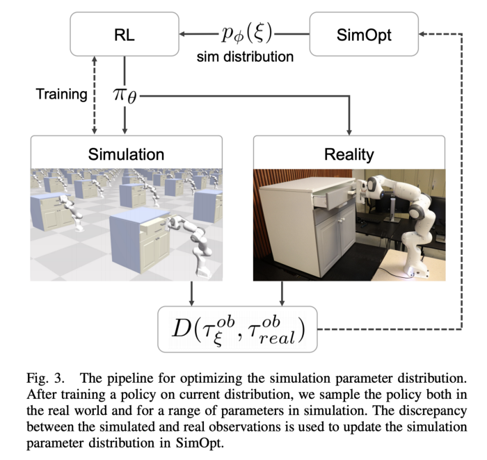
Overview of SimOpt

Just to recap domain randomization tries to find θ (the policy parameters) such that the same policy generalizes across several randomizations ξ ∈ P_ϕ of simulator dynamics.

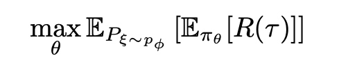
R(τ) is reward of the trajectory τ generated by running the policy π(θ)

SimOpt tries to minimize the following objective w.r.t simulator parameters ϕ

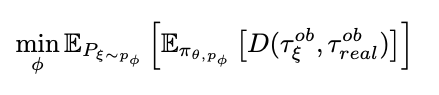
D is the discrepancy measure between simulated trajectory and real trajectory when running the policy π(θ). In this paper this is weighted average of L1 and L2 distances.

To reduce the amount of real world robot execution ϕ is only updated after a policy has fully converged in simulation. The iterative updates to ϕ is done as follows:

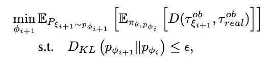
D_KL constraint is used to ensure the stability of optimization.

Here is the full algorithm for SimOpt:

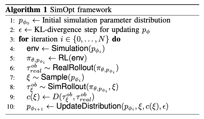
The number of iterations of sim-opt iteration is just N=3 iterations.

Here are some details of simulator randomizations. Let’s look at swing peg in hole task:

Simulator: NVIDIA FleX

Simulation Randomizations:

Swing peg in hole tasks:

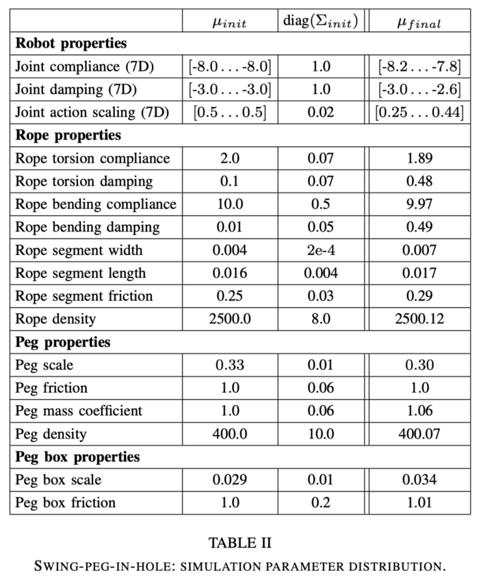
The adaptation of above simulation parameter covariance matrix and corresponding states at the end policy after fully trained.

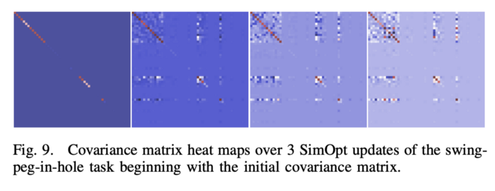
The 1st is the initialization of covariance matrix.

Although simulation parameters are quite exhaustive the policy inputs are quite minimal. 7 DoF joint positions and 3D position of the peg are inputs to the policy. The reward function is combination of distance from peg from hole, the angle alignment with hole and task success.

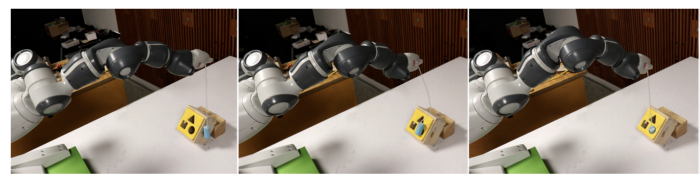
The fact that SimOpt needs to run the real robot execution in the training loop seems like it’s asking for a lot. However, notice that no reward function / no full state observations are needed in the real world execution step. All that is needed is to just run the learnt policy on the real robot. This seems like on the fly system identification such that policy trained on P_ϕ(ξ) generalizes on real robot.

The video below shows execution of policy trained via SimOpt

Conclusion:

We have seen several examples of successful transfers of sim2real for perception, grasping and feedback control policies. In all the examples, a lot of care has been taken to make the simulation as realistic as possible and choosing the parameters to randomize over. We also saw examples of guided domain randomizations, that simplify the task of manual tuning during sim2real transfer and avoids the policy convergence issues due to extra wide policy specifications.

Finally, will leave you with a comic (or a cautionary tale ?)

PC: https://twitter.com/dileeplearning

Sim2real For Robotic Manipulation